Lucky Numbers and Science

Earlier this week, Heiko Dudzus posted this challenge post on Dev.to. The challenge was this:

Write a program or script in your language of choice, that prints the lucky numbers between 1 and n. Try to make it as fast as possible for sieving lucky numbers between 1 and a million. (Perhaps it is sensible to measure the time without printing the results.)

A lucky number is defined as a number that survives the Sieve of Josephus. I’m going to quote the original post here so you get the idea.

The 1 is lucky by definition.

The successor of 1 is 2. So, every second number gets eliminated: 1, 3, 5, 7, 9, 11, 13, 15, 17, 19, 21, …

The next number is 3. Now, every third number gets eliminated: 1, 3, 7, 9, 13, 15, 19, 21, …

Number 3 is lucky! It’s successor is 7. Now, every seventh number gets eliminated. And so on.

See the link above for more details. I advise you to give the challenge a try if you haven’t yet before you read the rest of the post, since I’m about to tell you about my solutions.

I came up with two solutions, but the best solution ended up being an interesting combination of them both. You’ll see what I mean.

Solution 1: Naively Run the Algorithm

I like the quote “Make it work, make it right, make it fast”, which, as far as I can tell, this is attributed to Kent Beck. Therefore, my first solution focused on coding things exactly like the problem was provided, the easy way, whether or not this was the fastest way.

def lucky_numbers(max)
  possibles = (1..max).to_a
  1.step do |current_index|
    break if current_index >= possibles.size

    step_size = possibles[current_index]
    possibles = reject_every_nth_item(possibles, step_size)

    # If current_index is one of the items to get wiped out
    # the same current index will actually point at the next
    # number.  Reuse this index.
    redo if wiped_out?(ind, step_size)
  end
  possibles
end

def reject_every_nth_item(items, n)
  items.reject.each_with_index do |_, ind|
  	((ind + 1) % n).zero?
  end
end

def wiped_out?(ind, step_size)
  ((ind + 1) % step_size).zero?
end

I was all proud of myself as I ran it. And then I ran it with max = 1_000_000. And I sat. And I sat…

This is taking too long! I could to do better.

Solution 2: Focus on the Keeps, not the Rejects

As I was experimenting and testing things out, I noticed that, at the higher values of step_size, the naive algorithm was only rejecting a number every so often. So I thought to myself, “What if we could take the step size out of the equation and make each step take roughly the same amount of time, regardless of how many elements there were in it?” So, instead of checking each item to see if it was a reject, I calculated out the size of the chunk of non-rejected numbers and copied those into a results array, ignoring the rejects instead of explicitly rejecting them.

def lucky_numbers(max)
  possibles = (1..max).to_a
  1.step do |current_index|
    break if current_index >= possibles.size

    step_size = possibles[current_index]
    possibles = grab_chunks_between_rejects(possibles, step_size)

    redo if wiped_out?(current_index, step_size)
  end
  possibles
end

def grab_chunks_between_rejects(items, n)
  chunk_count = (items.size / n).floor

  # The new array will be the same size minus one reject item
  # for every chunk possible
  result = Array.new(items.size - chunk_count)
  chunk_target_index = 0

  # Some tricky indexing...
  # 1) Select chunks of size n - 1 (so as to not include the reject endpoint)
  # 2) Copy it into the results array
  # 3) Continue, each chunk after the one in front of it.
  (0...items.size).step(n) do |chunk_start|
  	chunk = items[chunk_start...(chunk_start + n - 1)]
    result[chunk_target_index...(chunk_target_index + chunk.size)] = chunk
    chunk_target_index += chunk.size
  end
  result
end

def wiped_out?(ind, step_size)
  ((ind + 1) % step_size).zero?
end

This one worked great! Even on my little laptop, it ran relatively quickly (don’t worry, the benchmarks are coming). But something felt weird. My programmer senses were tingling.

I had no proof at this point, but it seemed like all of the setup and creation of a second array each “round” should cause this algorithm to perform poorly at small step_sizes. It was at this point that this ceased to be a code challenge and became a science experiment.

Solution 3: A Combination of the Two

HYPOTHESIS: There is a performance trade-off between the low and high end for my two solutions. Thus, there should be a combination of the two that is faster than either one as a stand-alone.

If there was a trade-off somewhere between the two solutions, I would be able to run a few tests and find the best possible combination. I quickly updated my lucky_numbers method.

def lucky_numbers(max, strategy_switch = 10)
  possibles = (1..max).to_a
  1.step do |current_index|
    break if current_index >= possibles.size

    step_size = possibles[current_index]

    # Calculate next round of numbers
    possibles = if step_size <= strategy_switch
                  reject_every_nth_item(possibles, step_size)
                else
                  grab_chunks_between_rejects(possibles, step_size)
                end

    redo if wiped_out?(current_index, step_size)
  end
  possibles
end

And now to collect some data! For sanity’s sake, I wrapped each function in a module to differentiate them.

require "benchmark"

require_relative "lucky_numbers3"

max_nums = 1_000_000
switch_levels = [
  2,
  10,
  100,
  500,
  1000,
  5000,
  10_000,
  50_000,
  100_000,
  500_000,
]

Benchmark.bm do |bm|
  switch_levels.each do |level|
    bm.report(level.to_i) do
      Lucky3::lucky_numbers(max_nums, level)
    end
  end
end

# ▶ ruby optimize_lucky3.rb
#        user     system      total        real
#      2 17.550718  21.655086  39.205804 ( 39.535233)
#     10 18.351711  23.234818  41.586529 ( 42.615220)
#    100 18.443557  22.266405  40.709962 ( 41.178138)
#    500 20.278373  23.325708  43.604081 ( 44.987643)
#   1000 20.725864  22.510307  43.236171 ( 43.617160)
#   5000 27.245503  21.725938  48.971441 ( 49.304915)
#  10000 33.828295  22.476806  56.305101 ( 56.742865)
#  50000 82.069851  37.399753 119.469604 (120.174670)
# 100000 120.410101  23.425739 143.835840 (144.841090)
# 500000 445.835956  31.520488 477.356444 (483.688845)

And no science experiment is complete without plots! Unfortunately, the data visualization story (outside of the web) is not as cushy in Ruby as it is in Python. Fortunately, I found a wrapper for Python’s matplotlib so I could stay in Ruby land for now. Note that I used a log-based scale on the X-axis to better display my results.

# plot_lucky3.rb

require "matplotlib/pyplot"

plt = Matplotlib::Pyplot

xs = [2, 10, 100, 500, 1000, 5000, 10_000, 50_000, 100_000, 500_000]
ys = [
  39.54,
  42.62,
  41.18,
  44.99,
  43.62,
  49.30,
  56.74,
  120.17,
  144.84,
  483.69,
]
ax = plt.gca()
ax.scatter(xs, ys)
ax.set_xscale('log')
plt.show()

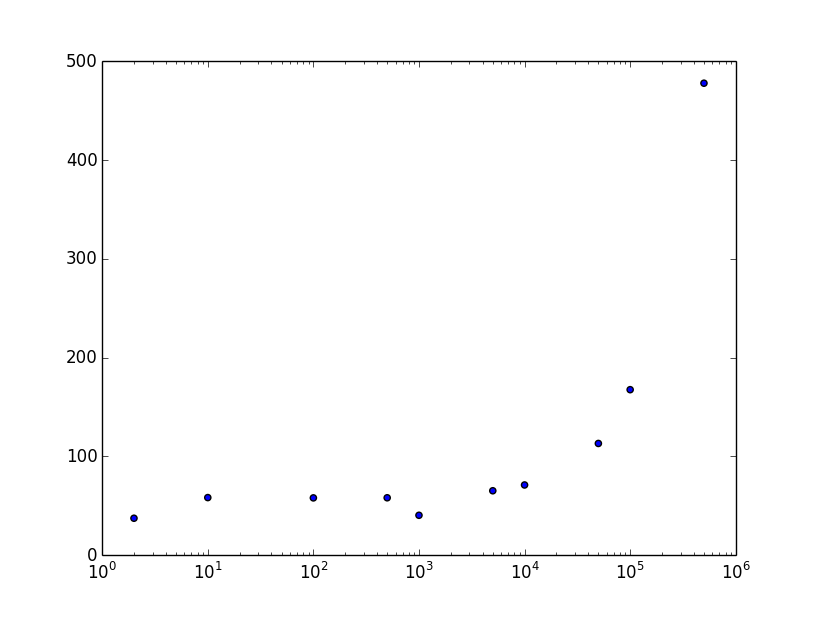
This is the part that is confusing to me. I’ve run the experiment multiple times and I always end up with a dip at around 1000. We’ll talk about that in a moment. Here are the benchmarks of each solution directly compared.

require "benchmark"

require_relative "lucky_numbers"
require_relative "lucky_numbers2"
require_relative "lucky_numbers3"

iterations = 1_000_000

Benchmark.bm do |bm|
  bm.report("Version 1") do
    Lucky1::lucky_numbers(iterations)
  end

  bm.report("Version 2") do
    Lucky2::lucky_numbers(iterations)
  end

  bm.report("Version 3") do
    Lucky3::lucky_numbers(iterations, 1000)
  end
end

And the results:

▶ ruby lucky_number_timer.rb
          user        system    total      real
Version 1 794.304851  28.946642 823.251493 (826.377494)
Version 2  23.267372  33.858966  57.126338 ( 57.238392)
Version 3  19.517162  20.816684  40.333846 ( 40.470201)

Conclusion

CONCLUSION: My hypothesis was supported. A combination of the two solutions performs better than either one solution by itself. However, the reason behind this is probably not the one that I initially thought. Some further research is required to find out why this worked.

My wife teaches middle school science and I just got done helping her judge their science fair, so I’ve got experimentation on the brain. Hopefully this little experiment makes her proud!

I’m sure my solution wasn’t the best possible solution, but it gets the job done. Ruby isn’t necessarily the language of choice for high-throughput calculations (although it’s not necessarily a bad choice either). If anybody can come up with a convincing reason for why my data came out the way it did, including the dip at 1000, I’ll personally send you a shiny new trophy emoji. 🏆 Also, if you’ve got a solution that you like better than these, I want to see it. Share it! (or share a link to your solution commented on Heiko’s original post).

Author: Ryan Palo | Tags: ruby puzzle performance | Buy me a coffee

Like my stuff? Have questions or feedback for me? Want to mentor me or get my help with something? Get in touch! To stay updated, subscribe via RSS