Data Science Cardio 1 - Weather
2464 words. Time to Read: About 24 minutes.I’m going to shamelessly borrow the idea of programming cardio from Wes Bos’s JavaScript30 course. I thought you folks might like it if I present a short data science example problem and then work through it with you. I’ve got a student learning Python that I’m tutoring right now (my first one! Yay!), and this was one of her problems. It seemed like an example that covered a lot of bases. This example will be in Python (3). I’ll try to link to the appropriate libraries and docs when they come up so you can explore further instead of taking my word for things.
So, without further ado, let’s. Get. PUMPED!
0. The Problem
We have been asked to investigate how various weather phenomena vary based on latitude. Specifically, we need to collect at least 500 samples of weather data, randomly distributed across the globe. Once we have this data, we should create plots and comment on any patterns we see in Temperature, Humidity, Cloudiness, and Wind Speed. I’m going to convert to the US customary system of units. You do whatever makes you happy.
A note: there are a bunch of different ways you could go about solving this problem. I’m going to show you one way. Feel free to explore your own solution method and see if the results turn out similar.
A second note: I use a few libraries that aren’t a part of the standard library, but are available in the Python Package Index (PyPI). If you come up against a No module named 'whatever' error, you’ll need to open up a terminal window and type pip install <packagename>, where <packagename> is the name of the package you’re missing, and hit Enter. Optionally, if you’re using Jupyter Notebooks, you can also type ! pip install <packagename> in a cell and run it. The bang (!) lets the notebook run a one-line system call.
I initially completed this analysis using a Jupyter Notebook. I highly recommend that. You can find the source code repo here if you get antsy and want to peek ahead.
1. 500 Random Coordinates
The first thing we need is 500 random coordinates. We’ll need these numbers to span across the whole range of possible latitudes (-90 degrees to 90 degrees), as well as the whole range of possible longitudes (-180 degrees to 180 degrees). Note that negative latitude indicates South, and negative longitude indicates West.
import numpy as np
import pandas as pd

np.random.seed(125)  # So that other scientists can duplicate our work!
lats = np.random.randint(-90, 90, size=500)
longs = np.random.randint(-180, 180, size=500)
coords = pd.DataFrame({
    "latitude": lats,
    "longitude": longs
})

# Let's take a look at how our coordinates look
coords.head()
| latitude | longitude | |
|---|---|---|
| 0 | 67 | -117 |
| 1 | -3 | 11 |
| 2 | -23 | -146 |
| 3 | 20 | -19 |
| 4 | -47 | 6 |
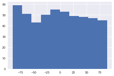
For sanity’s sake, let’s ensure our coordinates are reasonably random.
from matplotlib import pyplot as plt
# And, we're going to give our plots a bit of pizazz.
# Feel free to skip these two lines
import seaborn

seaborn.set()

plt.hist(coords['latitude'])
plt.show()
plt.hist(coords['longitude'])
plt.show()
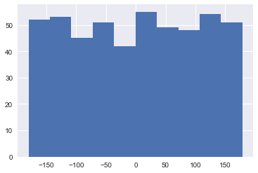
There are some spikes, but overall, it seems reasonable for what we’re doing. If you’re unhappy with the random-osity of your data, go ahead and change the random seed and re-run the cells above.
2. Setting Up the Weather API
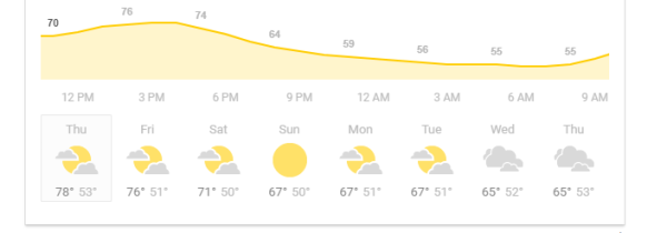
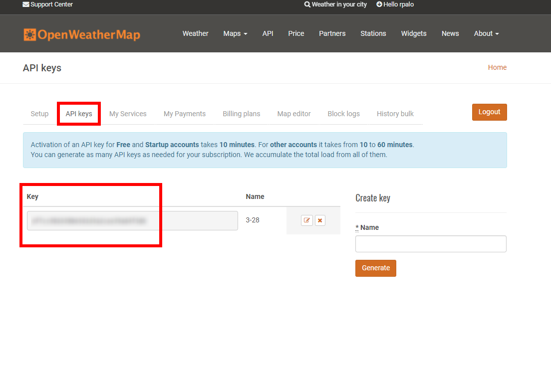
This part is going to be more administrative and less fun programming. But that’s OK! In order to get this weather data, we’ll need to hit a web API and ask it for the data. Specifically, we’re going to be using the OpenWeatherData API. You’ll need to create an account (it’s free!) and you’ll be provided with an API key, which you can find on the “API Keys” tab of your account page.
Keep this key a secret (I’ll give you some pointers on how to do this well). You wouldn’t want some nefarious person hammering the weather API and everybody thinking it was you. Think about your reputation as a good weather API citizen! Think of the children!
As the page says, it may take a little while before your key is working. Luckily, we’ve got some setup to do before we’re ready to make use of it. For now, let’s take a look at the endpoint we’ll be using. Check out the coordinate weather endpoint docs.
We could ask for the data we need in a few different ways, but since we’ve already created a bunch of beautiful (latitude, longitude) pairs, I think that’s probably the easiest way to go.
http://api.openweathermap.org/data/2.5/weather?lat={lat}&lon={lon}&APPID={api_key}
You’ll notice that, even though the online documentation doesn’t discuss it right there, we’ll need to add the APPID parameter with our API key. If you’re feeling really cool, you can also add units=imperial to get Fahrenheit temperature and Miles/Hour wind speed. You can also stick to the defaults and convert later. I’ll show you that process as well. Now, enough administrative stuff! Let’s get back to the code!
3. Setting Up to Get the Data
Before we open up our analysis code, I recommend you open a new file in the same directory called secrets.py.
# secrets.py
API_KEY = "copy your api key here"
If you’re keeping track of this project with a git repository, add this file to your .gitignore file.
__pycache__/
.ipynb_checkpoints
secrets.py
haters
Now we’re ready to dive back into the notebook.
from secrets import API_KEY
import requests
import time

def get_weather_data(coords, time_between=1):
    """Queries the OpenWeatherAPI for data.

    Args:
    	coords: A Pandas DataFrame with rows containing 'latitude'
    		and 'longitude' columns.
    	time_between: An integer specifying the sleep time in seconds
    		between each API ping.  Defaults to the OpenWeatherAPI's
    		recommended limit of 1 request per second.

    Returns:
    	A list of nested dicts (loaded JSON results).
    """
    results = []
    for ind, row in coords.iterrows():
        lat, lon = row['latitude'], row['longitude']
        query = f"http://api.openweathermap.org/data/2.5/weather?lat={lat}&lon={lon}&APPID={API_KEY}"
        response = requests.get(query)
        results.append(response.json())
        time.sleep(time_between)
    return results
There are two key features to this code. The first is the “f-string”, which is Python 3’s shwoopy syntax for string interpolation. The nice thing is that these “f-strings” are super fast! Relatively speaking, at least. But we are able to insert our latitude and longitude values directly from the DataFrame row, as well as our API key.
The other key feature is that we’re using requests to make a get request, and then using the json function to immediately process the response into a Python dict we can work with. If you weren’t sure how we were going to get the data from the API, you might actually be disappointed that it’s not more complicated than this. As long as you know the right URL, requests makes our job pretty darn pleasant.
3a. Logging our Requests
I’m going to go on two quick asides for some extra practice. If you want to skip right to step four, don’t worry. You won’t hurt my feelings.
The first aside I’m going to go on is to set up some logging to a file. Up towards the top of your notebook, add the following code.
import logging

logger = logging.getLogger('weather')
logger.setLevel(logging.INFO)
fh = logging.FileHandler('api_calls.log')
formatter = logging.Formatter('%(asctime)s - %(message)')
fh.setFormatter(formatter)
logger.addHandler(fh)
And then inside your get_weather_data function:
def get_weather_data(coords, time_between=1):
    # ...
    results = []
    for ind, row in coords.iterrows():
        lat, long = row['latitude'], row['longitude']
        query = f"http://api.openweathermap.org/data/2.5/weather?lat={lat}&lon={lon}&APPID={API_KEY}"

        # Here's the new stuff
        clean_url = query.rpartition("&")[0]  # Don't log your api key!
        logger.info(f"Call {ind}: ({lat}, {lon}) - {clean_url}")

        response = requests.get(query)
        results.append(response.json())
        time.sleep(time_between)
    return results
Now we get to save a log of all the URL’s we hit!
3b. Getting the Closest City Name
You know what would be nice? Logging out the name of the closest city with our logs. There’s a neat little library called citipy that does just that! Let’s update our get_weather_data function one more time.
from secrets import API_KEY
from citipy import citipy  # Make sure to import it once you've installed it

def get_weather_data(coords, time_between=1):
    # ...
    results = []
    for ind, row in coords.iterrows():
        lat, lon = row['latitude'], row['longitude']
        query = f"http://api.openweathermap.org/data/2.5/weather?lat={lat}&lon={lon}&APPID={API_KEY}"
        clean_url = query.rpartition("&")[0]

        # Here's the new stuff
        city = citipy.nearest_city(lat, lon)
        logger.info(f"Call {ind}: {city.city_name} {clean_url})")

        result = requests.get(query)
        results.append(result.json())
        time.sleep(time_between)
    return results
This will be great! Back to the problem at hand.
4. Actually Getting Our Data
Let’s test our function with a test call, first.
test_coords = pd.DataFrame({"latitude": [37], "longitude": [-122]})
test_results = get_weather_data(test_coords)
test_results
[{'base': 'stations',
  'clouds': {'all': 1},
  'cod': 200,
  'coord': {'lat': 37, 'lon': -122},
  'dt': 1522341300,
  'id': 5381421,
  'main': {'humidity': 76,
   'pressure': 1021,
   'temp': 287.78,
   'temp_max': 289.15,
   'temp_min': 286.15},
  'name': 'Pasatiempo',
  'sys': {'country': 'US',
   'id': 399,
   'message': 0.004,
   'sunrise': 1522331815,
   'sunset': 1522376913,
   'type': 1},
  'visibility': 16093,
  'weather': [{'description': 'clear sky',
    'icon': '01d',
    'id': 800,
    'main': 'Clear'}],
  'wind': {'deg': 331.003, 'speed': 1.32}}]
If yours comes out just like mine, then it looks like we’re good to run the full data collection.
full_results = get_weather_data(coords)
full_results[:3]  # Let's peek at the first 3 datapoints
This will run for about 8 and a half minutes (the cost of being a good citizen). Go get a coffee or a snack to reward yourself for all your hard work.
5. Saving the Data
First thing’s first. Let’s save our data out so we’ll have it just in case something gets exploded.
import json

with open("weather.json", "w") as outfile:
    json.dump(full_results, outfile)
This will create a new file weather.json in your project directory. Time for another optional side-step: unit conversion.
5a. Unit Conversion
If you didn’t use the units=imperial parameter in your API call and you want US customary units, you’ll need some helper functions.
def k_to_f(temp):
    """Converts a Kelvin temperature to Fahrenheit"""
    return temp * 9/5 - 459.67

def mps_to_mph(speed):
    """Converts a meters/s speed to miles/hour"""
    return speed * 2.23694
6. Munging the Data
Yes, it’s a word. Look it up. Whatever. We’re going to need to build a data structure that we can turn into a DataFrame, and we want to narrow things down to just the data we care about. Take another look at your example output above and dig into the JSON data.
important_json_data = []
for point in full_results:
    lat = point['coord']['lat']
    lon = point['coord']['lon']
    temp = k_to_f(point['main']['temp'])
    humidity = point['main']['humidity']
    cloudiness = point['clouds']['all']
    wind = mps_to_mph(point['wind']['speed'])

    row = [lat, lon, temp, humidity, cloudiness, wind]
    important_json_data.append(row)

weather_df = pd.DataFrame(important_json_data)
weather_df.columns = [
    "latitude",
    "longitude",
    "temperature",
    "humidity",
    "clouds",
    "wind",
]
weather_df.head()
| latitude | longitude | temperature | humidity | clouds | wind | |
|---|---|---|---|---|---|---|
| 0 | 67 | -117 | -16.15 | 69 | 8 | 4.29 |
| 1 | -3 | 11 | 74.93 | 96 | 68 | 2.17 |
| 2 | -23 | -146 | 80.96 | 100 | 88 | 12.91 |
| 3 | 20 | -19 | 67.37 | 100 | 8 | 9.78 |
| 4 | -47 | 6 | 44.78 | 97 | 8 | 13.35 |
Again, let’s save our data out just in case.
weather_df.to_csv("weather.csv")
Congratulations! The heavy lifting is done. Let’s take a look at our data and see what conclusions we can draw.
7. Plotting the Data
Remember our goals?
- Compare temperature and latitude.
- Compare humidity and latitude.
- Compare cloudiness and latitude.
- Compare wind speed and latitude.
- Draw some conclusions.
I’m going to put the latitude on the Y-axis, because I feel like the plots will feel more intuitive. We generally think about latitudes going North to South and thus top to bottom. If you want to insist on plotting the independent variable (latitude) on the X-axis and the dependent variable (temperature) on the Y-axis, then do whatever makes you happy.
Temperature
plt.scatter(weather_df.temperature, weather_df.latitude)
plt.xlabel("Temperature (F)")
plt.ylabel("Latitude (degrees)")
plt.title("Temperature vs. Latitude")
plt.show()
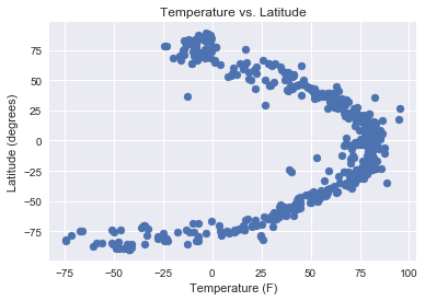
Woohoo! That’s some strong trending right there! As you might have expected, the temperature climbs as you approach the equator and drops off as you near the poles. Go science!
Humidity
plt.scatter(weather_df.humidity, weather_df.latitude)
plt.xlabel("Humidity (%)")
plt.ylabel("Latitude (degrees)")
plt.title("Humidity vs. Latitude")
plt.show()
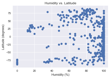
These are some strange results. It looks like, except for a few drop offs, an abundance of the data points had 100% humidity. I find this hard to believe. I found a few Google results that make me wonder if there’s not something weird with the way that they’re measuring humidity. If anybody has any other thoughts, I’d be interested to hear them. Let me know what you think.
Cloudiness
plt.scatter(weather_df.clouds, weather_df.lat)
plt.xlabel("Cloudiness (%)")
plt.ylabel("Latitude (degrees)")
plt.title("Cloudiness vs. Latitude")
plt.show()
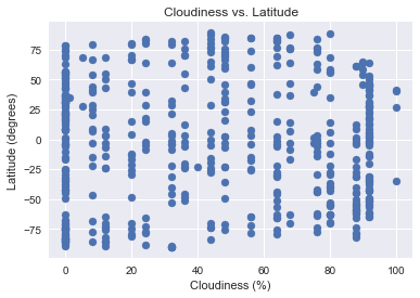
I can’t really see much of a trend here, either. The striation of the data (neat rows) makes me feel like there’s some kind of a pattern, though. Let’s see if maybe there’s a longitude relationship.
plt.scatter(weather_df.long, weather_df.clouds)
plt.xlabel("Longitude (degrees)")
plt.ylabel("Cloudiness (%)")
plt.title("Longitude vs. Cloudiness")
plt.show()
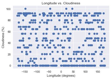
Hmm… I’m still not seeing much of a relationship. Once again, if anybody has any thoughts, let me know!
Wind Speed
plt.scatter(weather_df.wind, weather_df.lat)
plt.xlabel("Wind Speed (mph (abs))")
plt.ylabel("Latitude (degrees)")
plt.title("Wind Speed vs. Latitude")
plt.show()
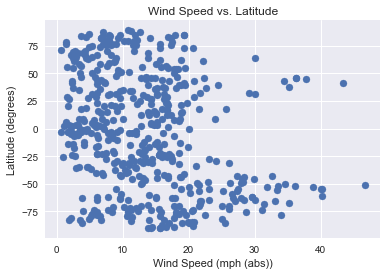
This is an interesting plot. We see kind of a mish-mash, but with some clear spikes at about -50 degrees and 50 degrees. It seems to drop off toward zero around the poles and the equator. At first, I was confused, but then I remembered my 8th grade science class.
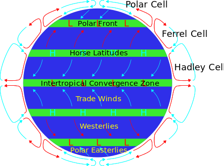
There are a group of winds called the “Westerlies” that blow between 40 and 50 degrees North and South latitude. These are sometimes called the “Roaring Forties” and, due to the expanses of open ocean in the southern hemisphere especially (no land or trees to impede the winds), they are used to speed up sailing times. They tend to shift towards the equator in that hemisphere’s summer and towards the pole in the winter.
Conversely, the area around the equator is known as the “Intertropical Convergence Zone,” also called the “doldrums.” This area is a combination of dead wind and thunderstorms, depending on season.
I feel reasonably comfortable saying our data seems to support this trend. And so, once again, hooray for science!
Wrap Up
That’s it! Hopefully you enjoyed the practice. If you come up with any other neat findings from our data, be sure to share them with me.
Happy munging!
Author: Ryan Palo | Tags: python data-science scientific tutorial |Like my stuff? Have questions or feedback for me? Want to mentor me or get my help with something? Get in touch! To stay updated, subscribe via RSS